
Assumptions / Validation

Model Assumptions and Validation
HNN is designed to be a tool from which multi-scale testable predictions on the cell and circuit mechanisms generating source-localized M/EEG signals can be made. An advantage of interpreting signals in source space is that HNN does not need to account for the mixing of signals from many regions that contribute to sensor signals, rather this is accounted for using source estimation (e.g., MNE-Python). HNN has been successfully used to develop testable predictions on the multi-scale mechanisms underlying source localized event-related potentials (ERPs) and low-frequency brain rhythms in various experimental conditions (See publications page).
Here, we provide further information about the assumptions built into the HNN Template Model and into the workflows of use in our tutorials on how to begin to study the mechanisms creating ERPs and low frequency brain rhythms. We highlight some of the literature that supports these assumptions and emphasize that HNN is a tool to develop testable predictions on the origin of these signals, which may be different depending on the experimental conditions. We also describe the process for defining and testing hypotheses and for estimating parameters in HNN. Lastly, we describe the process for validating that the multi-scale model-derived predictions are true in the brain.
Assumptions Built in the HNN Template Model and Tutorial Workflows
HNN Template Model Assumptions
While the HNN Template Model includes biophysical details, it still represents a reduced representation of the full complexity of neocortical circuits. If and how much the finer details of neocortical cells and circuits contribute to macro-scale M/EEG, potential differences across brain areas and species are unknown. The goal of HNN is to provide a tool where testable predictions can be developed and built upon starting with well-established general principles on the canonical nature of neocortical circuitry. As further knowledge is gained, HNN can be adapted to include greater detail.
It is well-established that the current flow in the large and spatially aligned cortical pyramidal neuron dendrites is the main generator of primary current dipoles1–6. As such, HNN simulates the averaged equivalent current dipole in a region of interest from a neocortical column model via the net intracellular electrical current flow in the pyramidal neuron dendrites multiplied by their length (see red/green arrows in Fig. 1)1–6. This calculation produces physical units of current x distance (nano-Ampere-meter, nAm) that are directly comparable to source localized M/EEG units (e.g. Fig. 2 bottom left and Fig. 3A/B below).
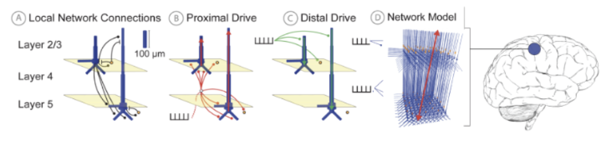
HNN’s foundational neocortical column model, referred to as the HNN Template Model (Fig. 1), was developed based on canonical principles of neocortical circuitry and contains minimal circuit elements essential to generating primary current dipoles and connecting to layer and cell-specific neocortical activity2, and at a scale tractable to be run on a laptop. Details of the model can be found on the HNN Template model page. In brief, the model contains multi-compartment pyramidal neurons in the supragranular (L 2/3) and infragranular layers (L 5) and single-compartment inhibitory neurons in each layer. The morphology and physiology of the neurons and connectivity among the cells were based on empirical data and prior published models, as detailed in earlier publications2,7,8.
Further, to represent input to the local network from thalamic or other cortical areas (not explicitly modeled), HNN includes methods to define trains of action potentials in predefined temporal patterns (e.g. see example and histograms in Fig. 2) that activate layer-specific excitatory synapses. These drives represent “feedforward” (proximal) and “feedback” (distal) drives, and their post-synaptic targets within the cortical layers are based on well-established connectivity rules9–14.
ERP and Low Frequency Rhythm Tutorial Workflow Assumptions
All simulation experiments consist of activating the cortical template model with exogenous feedforward or feedback input, or noise, depending on the experimental conditions you are studying. HNN-GUI tutorials (and corresponding HNN-Core tutorials) are designed to teach users how to activate the network with patterns of exogenous spiking input and noise to study ERPs and low-frequency rhythms. Our tutorials are based on our prior published studies where we developed predictions on the cell and circuit mechanisms underlying ERPs and low-frequency rhythms and differences across experimental conditions. These prior studies were motivated by a long history of research, mainly in animals, investigating the neural mechanisms of ERPs and low-frequency rhythms (see extensive references e.g. ERPs7,15 e.g. alpha rhythms8,16–19, e.g. beta rhythms8,17,19,20e.g. gamma rhythms17,21–24). HNN allowed us to test if the cell and network elements thought to be the primary generators of these signals based on animal research (e.g. a sequence of thalamocortical drive to the network) could produce macro-scale current dipole signals that were in agreement with our recorded data. While the literature guided us to a starting point that constrained the investigation, the exact parameters to use to present the data were unknown. By directly comparing the current dipole output of the model to source localized empirical data, we were able to titrate parameters (both through hand tuning and algorithmic parameter estimation) to produce a close fit to the source waveform (i.e. small root mean squared error (RMSE)). Once a close fit to the current dipole waveform was established the model provided a number of testable predictions on the underlying cell and circuit activity, i.e. exogenous input timing and strength, cell spiking activity, LFP/CSD, etc. An example of this hypothesis testing and parameter tuning process is described further below.
We provide a pre-tuned model along with data and parameter sets from our published studies for users to begin with (e.g., see Fig. 2) and teach users the workflow we used to study the multi-scale origin of these signals. The pre-tuned network and exogenous input parameters distributed with HNN have been a successful starting point for many studies (See Publications). The model and workflows are meant as a starting point for how to use HNN to generate testable predictions and not to propagate singular theories on signal generation. See below for further details on how to test that model-derived predictions are valid in the real brain.
HNN provides a pre-tuned neocortical column model and tutorials on how to begin to activate the model with exogenous thalamocortical and cortical-cortical drive as described above. In practice, users start with hypotheses about how the network is activated during the experimental conditions they are studying (e.g. sequence of feedforward and feedback drive), and test if and how the parameters representing this activation (e.g. strength of distal input to layer ⅔ pyramidal vs inhibitory cells) can be adjusted to get an accurate representation of the source data. If they can, then the “tuned” model provides multi-scale testable predictions on the underlying cell and network activity creating the signal. If they can’t, alternative hypotheses can be tested. It may be that more than one set of parameter combinations (i.e. “models”) can provide a “good fit” to the data (defined below). As discussed above, currently in large-scale biophysically detailed models, we can not test all possible parameter combinations. In practice, most parameters are fixed based on best-known constraints and only a small number of parameters are estimated based on “testing hypotheses”. When using HNN, users often define a handful of logical hypotheses and identify the parameters that correspond to testing these hypotheses. Hypothesis testing in this context means that through parameter estimation (described further below) users determine if and how any of the targeted parameters is able to provide a better fit to the data. If more than one set of parameters generates a good fit to the data, by definition the underlying multiscale cell and circuit level activity will be different because they are defined by different parameters (i.e. “models”). These microcircuit differences provide targets for further model selection based on data from invasive animal recordings and/or other imaging methods, discussed further below.
Below, we give a concrete example of how hypotheses can be developed and tested in HNN, and compared to alternative hypotheses. First, we describe the parameter estimation process where the “goodness of fit” of the model is assessed by examining the root mean squared error (RMSE) between the simulated and empirical current source signals. An acceptable fit depends on the user-defined criteria on a good fit threshold. HNN does not currently provide tools for accessing the quality of the fit between model and source data beyond RMSE, nor does it provide a method for statistically comparing alternate models. Rather, the user can test multiple predictions and report the one that gives the closest fit (smallest RMSE) to the data. HNN also does not currently have methods to fit model parameters to other types of empirical data e.g. cell spike rate and/or LFP/CSD. Such method developments are ongoing and represent important future directions.
Parameter Estimation Process
Once a hypothesized pattern of drive to the local circuit representing the conditions of the experiment is determined, the process for adjusting parameters in HNN is as follows. Users first adjust parameters via exploration and “hand tuning” to get a sense of how parameter changes map onto multi-scale changes in the model. This sense comes from visually examining the multi-scale output in the HNN GUI, including directly comparing the source signals from the model and data. We can not emphasize enough the importance of hand tuning and exploration to understand how the model components contribute to the signal.
Once an initial close representation of the signal is found via hand tuning (i.e. small RMSE error between model and data current dipole waveforms), users can define a targeted set of parameters for algorithmic estimation of values that produce the “best fit to data” (determining the goodness of fit is defined above). Currently, HNN only has built-in parameter estimation tools for parameters of the exogenous drive during an evoked response simulation that employ a temporally-weighted loss function optimized using gradient-free solvers (see Optimization Tutorial). Additional parameter estimation methods are in the development phase.
Once a good first-to-one signal is determined, users may wish to next test hypotheses on the cell and circuit mechanisms underlying differences in signals across experimental conditions (e.g., see testing of hypotheses on differences in sensory-driven responses in typically developing children vs children with autism spectrum disorder25; or differences in auditory evoked responses across hemispheres15).
The final set of parameters that produce an accurate representation of the data provides predictions on the circuit activity at multiple scales (cell-specific spiking patterns, LFP/CSD.. etc). These predictions all provide targets for testing further in the real brain (see Fig 3 and section below).
Parameter Sensitivity
Once a “good fit” to data is found (defined above), the sensitivity of the fit to variation in model parameters can be made. HNN is not yet distributing tools for parameter sensitivity analysis. For an example of how to use the python package 'Uncertainty'36 to apply sensitivity analysis on parameters see the supplementary materials in the HNN methods paper (Neymotin et al eLife 2020). This example uses the method of variance-based sensitivity analysis through Monte Carlo estimation37 and provides Sobol sensitivity indices that can be used to explain the relative contribution of individual parameters on model variance. The total Sobol sensitivity index for each parameter serves as a measure that represents that parameter’s contribution to the variance, and also the contributions resulting from interactions with other parameters being varied38. So a parameter with a low total Sobol sensitivity index can be characterized as an insignificant contributor to variance and can be fixed at its default value during model optimization.
Example of how HNN can be used to develop and test hypotheses (see also alpha/beta tutorial)
A primary example of HNN’s utility in developing and testing hypotheses comes from our work studying the neural origin of the transient 15-29Hhz beta oscillations (e.g. beta events) observed in source-localized MEG signals from SI. Here, beta emerges as part of a rhythm that contains non-overlapping transient alpha and beta components and is known as the somatosensory “mu” rhythm8,19). We began with knowledge from prior studies of the circuit mechanisms underlying alpha and beta generation. A long history of research has shown that alpha rhythms can emerge from ~10Hz bursting in the thalamus that activates the cortex through layer-specific thalamocortical projections (see Hughes and Crunelli 200535 for review). Prior theories on beta generation, based mostly on slice experiments and modeling, suggested beta originates from fast synaptic interactions between excitatory and inhibitory neurons that act in concert with slow potassium currents (AHP currents) in excitatory neurons to pace the excitatory cells to fire regularly at a beta frequency17,32–34. HNNs Template Model contains the circuit elements needed to test if these mechanisms could account for alpha and beta events in our human MEG data. We began with parameter exploration and simulated 10Hz bursts of activity that activated the model via the thalamocortical projection pattern (i.e. proximal drive Fig. 1) and drove spiking in the cortical excitatory cells, which we predicted could in turn create the beta component of the rhythm through the local excitatory and inhibitory connections. Despite extensive parameter tuning efforts, we found that while alpha could be generated this way, we could not accurately simulate beta. Instead, by parameter exploration we found a completely novel mechanism that closely produced numerous quantified data features (Fig. 3 A/B8); this analysis was only possible because of the detail in the HNN template model that enabled a one-to-one comparison between model output and data in the same physical nAm units. This mechanism suggested that there were two distinct generators of 10Hz bursting activity, one that drove the network through the proximal projection pathway and one through the distal projection pathways (possibly representing activity in lemniscal and non-lemniscal thalamic nuclei ). When the bursts arrived asynchronous to the cortex alpha events emerged and when they arrived nearly synchronously beta events emerged8 (see also alpha/beta tutorial). Of note, while we examined variation in parameters, we did not perform automated parameter fitting or parameter sensitivity analyses in this study. This mechanism for alpha generation was consistent with prior studies (Bollimunta et al 2008) but represented a completely new theory on the generation of beta. Owing to HNN’s biophysical detail, additional testable predictions on the expected layer-specific LFP and CSD could be made. These predictions were detailed in19 and supported by laminar recordings in mice and monkeys (Fig. 3C), and later with high-resolution laminar MEG that also suggested a similar beta event mechanism occurs in the primary motor cortex26. Further model analysis with HNN-predicted beta events generated via these mechanisms may causally suppress tactile perception through the recruitment of supragranular inhibition20; this prediction is currently being tested with invasive animal recordings.
We are developing tools that can further facilitate this validation process, including expanded parameter estimation techniques that can constrain model output to multiple data types (e.g. spike rates, LFP/CSD). A key technique for validating model hypotheses is recording across the cortical layers (e.g. laminar recordings) as the source of human M/EEG signals necessarily relies on the integration of information across the layers.
In practice, the development and validation of model-derived predictions will take collaborative efforts between researchers with different expertise including human imaging researchers and clinicians, neural modeling experts, and neurophysiologist recording invasively in animal models. A goal of our HNN workshops and open-source modeling framework is to bring together researchers with varied backgrounds and expertise who are all interested in bridging the gap between human and animal research.
References
While the HNN Template Model includes biophysical details, it still represents a reduced representation of the full complexity of neocortical circuits. If and how much the finer details of neocortical cells and circuits contribute to macro-scale M/EEG, potential differences across brain areas and species are unknown. The goal of HNN is to provide a tool where testable predictions can be developed and built upon starting with well-established general principles on the canonical nature of neocortical circuitry. As further knowledge is gained, HNN can be adapted to include greater detail.
It is well-established that the current flow in the large and spatially aligned cortical pyramidal neuron dendrites is the main generator of primary current dipoles1–6. As such, HNN simulates the averaged equivalent current dipole in a region of interest from a neocortical column model via the net intracellular electrical current flow in the pyramidal neuron dendrites multiplied by their length (see red/green arrows in Fig. 1)1–6. This calculation produces physical units of current x distance (nano-Ampere-meter, nAm) that are directly comparable to source localized M/EEG units (e.g. Fig. 2 bottom left and Fig. 3A/B below).
Figure 1 HNN Template Model (A) Pyramidal (Pyr, Blue), interneurons (IN, orange), and local network synaptic connectivity. (B) Proximal input pathway relaying spiking information from thalamic sources through excitatory synapses on Pyr proximal dendrites (C) Distal input pathway relaying spiking to distal dendrites. (D) Full network model with an adjustable number of neurons: default is 100 Pyr & 33 IN per layer. A multiplicative scaling factor is applied to estimate the number of synchronous Pyr contributing to a recorded signal. Net current dipole is calculated from the Pyr dendritic current flow (red arrow).
HNN’s foundational neocortical column model, referred to as the HNN Template Model (Fig. 1), was developed based on canonical principles of neocortical circuitry and contains minimal circuit elements essential to generating primary current dipoles and connecting to layer and cell-specific neocortical activity2, and at a scale tractable to be run on a laptop. Details of the model can be found on the HNN Template model page. In brief, the model contains multi-compartment pyramidal neurons in the supragranular (L 2/3) and infragranular layers (L 5) and single-compartment inhibitory neurons in each layer. The morphology and physiology of the neurons and connectivity among the cells were based on empirical data and prior published models, as detailed in earlier publications2,7,8.
Further, to represent input to the local network from thalamic or other cortical areas (not explicitly modeled), HNN includes methods to define trains of action potentials in predefined temporal patterns (e.g. see example and histograms in Fig. 2) that activate layer-specific excitatory synapses. These drives represent “feedforward” (proximal) and “feedback” (distal) drives, and their post-synaptic targets within the cortical layers are based on well-established connectivity rules9–14.
ERP and Low Frequency Rhythm Tutorial Workflow Assumptions
All simulation experiments consist of activating the cortical template model with exogenous feedforward or feedback input, or noise, depending on the experimental conditions you are studying. HNN-GUI tutorials (and corresponding HNN-Core tutorials) are designed to teach users how to activate the network with patterns of exogenous spiking input and noise to study ERPs and low-frequency rhythms. Our tutorials are based on our prior published studies where we developed predictions on the cell and circuit mechanisms underlying ERPs and low-frequency rhythms and differences across experimental conditions. These prior studies were motivated by a long history of research, mainly in animals, investigating the neural mechanisms of ERPs and low-frequency rhythms (see extensive references e.g. ERPs7,15 e.g. alpha rhythms8,16–19, e.g. beta rhythms8,17,19,20e.g. gamma rhythms17,21–24). HNN allowed us to test if the cell and network elements thought to be the primary generators of these signals based on animal research (e.g. a sequence of thalamocortical drive to the network) could produce macro-scale current dipole signals that were in agreement with our recorded data. While the literature guided us to a starting point that constrained the investigation, the exact parameters to use to present the data were unknown. By directly comparing the current dipole output of the model to source localized empirical data, we were able to titrate parameters (both through hand tuning and algorithmic parameter estimation) to produce a close fit to the source waveform (i.e. small root mean squared error (RMSE)). Once a close fit to the current dipole waveform was established the model provided a number of testable predictions on the underlying cell and circuit activity, i.e. exogenous input timing and strength, cell spiking activity, LFP/CSD, etc. An example of this hypothesis testing and parameter tuning process is described further below.
We provide a pre-tuned model along with data and parameter sets from our published studies for users to begin with (e.g., see Fig. 2) and teach users the workflow we used to study the multi-scale origin of these signals. The pre-tuned network and exogenous input parameters distributed with HNN have been a successful starting point for many studies (See Publications). The model and workflows are meant as a starting point for how to use HNN to generate testable predictions and not to propagate singular theories on signal generation. See below for further details on how to test that model-derived predictions are valid in the real brain.
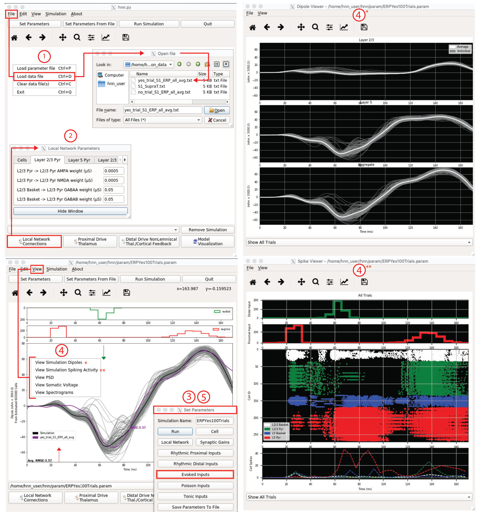
Figure 2 HNN GUI with example workflow to study the origin of an ERP. 1. Load data (purple, bottom left), 2. Adjust local network, if desired. 3. Define driving input histograms from exogenous brain areas. 4. Run simulation and view, current dipole (gray), layer-specific responses (upper right) & individual cell spiking (bottom right). Other visualization not shown. 5. Adjust parameters by exploration followed by optimization algorithms minimizing RMSE.
Process for Defining and Testing Hypotheses and Parameter Estimation
Working with large-scale neural models is challenging because not all parameters can be estimated at once. While one might want to simply feed in a waveform and have the model spit out all the possible parameter combinations that can create this waveform, at this time, that is not possible in HNN or in any large-scale neural modeling framework. There are simply too many parameters and possible parameter combinations. In practice, pieces of the model (e.g. individual cells and synaptic connections) are developed and parameters are tuned and fixed based on best-known biophysical constraints (e.g. morphology and physiology). Once an acceptable representation of elements of the model is developed, most parameters are fixed and parameter tuning and estimation are performed on a limited targeted set of parameters to test hypotheses on if and how those parameters contribute to specific signals of interest and changes in the signal across experimental conditions/subjects.HNN provides a pre-tuned neocortical column model and tutorials on how to begin to activate the model with exogenous thalamocortical and cortical-cortical drive as described above. In practice, users start with hypotheses about how the network is activated during the experimental conditions they are studying (e.g. sequence of feedforward and feedback drive), and test if and how the parameters representing this activation (e.g. strength of distal input to layer ⅔ pyramidal vs inhibitory cells) can be adjusted to get an accurate representation of the source data. If they can, then the “tuned” model provides multi-scale testable predictions on the underlying cell and network activity creating the signal. If they can’t, alternative hypotheses can be tested. It may be that more than one set of parameter combinations (i.e. “models”) can provide a “good fit” to the data (defined below). As discussed above, currently in large-scale biophysically detailed models, we can not test all possible parameter combinations. In practice, most parameters are fixed based on best-known constraints and only a small number of parameters are estimated based on “testing hypotheses”. When using HNN, users often define a handful of logical hypotheses and identify the parameters that correspond to testing these hypotheses. Hypothesis testing in this context means that through parameter estimation (described further below) users determine if and how any of the targeted parameters is able to provide a better fit to the data. If more than one set of parameters generates a good fit to the data, by definition the underlying multiscale cell and circuit level activity will be different because they are defined by different parameters (i.e. “models”). These microcircuit differences provide targets for further model selection based on data from invasive animal recordings and/or other imaging methods, discussed further below.
Below, we give a concrete example of how hypotheses can be developed and tested in HNN, and compared to alternative hypotheses. First, we describe the parameter estimation process where the “goodness of fit” of the model is assessed by examining the root mean squared error (RMSE) between the simulated and empirical current source signals. An acceptable fit depends on the user-defined criteria on a good fit threshold. HNN does not currently provide tools for accessing the quality of the fit between model and source data beyond RMSE, nor does it provide a method for statistically comparing alternate models. Rather, the user can test multiple predictions and report the one that gives the closest fit (smallest RMSE) to the data. HNN also does not currently have methods to fit model parameters to other types of empirical data e.g. cell spike rate and/or LFP/CSD. Such method developments are ongoing and represent important future directions.
Parameter Estimation Process
Once a hypothesized pattern of drive to the local circuit representing the conditions of the experiment is determined, the process for adjusting parameters in HNN is as follows. Users first adjust parameters via exploration and “hand tuning” to get a sense of how parameter changes map onto multi-scale changes in the model. This sense comes from visually examining the multi-scale output in the HNN GUI, including directly comparing the source signals from the model and data. We can not emphasize enough the importance of hand tuning and exploration to understand how the model components contribute to the signal.
Once an initial close representation of the signal is found via hand tuning (i.e. small RMSE error between model and data current dipole waveforms), users can define a targeted set of parameters for algorithmic estimation of values that produce the “best fit to data” (determining the goodness of fit is defined above). Currently, HNN only has built-in parameter estimation tools for parameters of the exogenous drive during an evoked response simulation that employ a temporally-weighted loss function optimized using gradient-free solvers (see Optimization Tutorial). Additional parameter estimation methods are in the development phase.
Once a good first-to-one signal is determined, users may wish to next test hypotheses on the cell and circuit mechanisms underlying differences in signals across experimental conditions (e.g., see testing of hypotheses on differences in sensory-driven responses in typically developing children vs children with autism spectrum disorder25; or differences in auditory evoked responses across hemispheres15).
The final set of parameters that produce an accurate representation of the data provides predictions on the circuit activity at multiple scales (cell-specific spiking patterns, LFP/CSD.. etc). These predictions all provide targets for testing further in the real brain (see Fig 3 and section below).
Parameter Sensitivity
Once a “good fit” to data is found (defined above), the sensitivity of the fit to variation in model parameters can be made. HNN is not yet distributing tools for parameter sensitivity analysis. For an example of how to use the python package 'Uncertainty'36 to apply sensitivity analysis on parameters see the supplementary materials in the HNN methods paper (Neymotin et al eLife 2020). This example uses the method of variance-based sensitivity analysis through Monte Carlo estimation37 and provides Sobol sensitivity indices that can be used to explain the relative contribution of individual parameters on model variance. The total Sobol sensitivity index for each parameter serves as a measure that represents that parameter’s contribution to the variance, and also the contributions resulting from interactions with other parameters being varied38. So a parameter with a low total Sobol sensitivity index can be characterized as an insignificant contributor to variance and can be fixed at its default value during model optimization.
Example of how HNN can be used to develop and test hypotheses (see also alpha/beta tutorial)
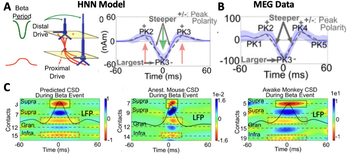
A primary example of HNN’s utility in developing and testing hypotheses comes from our work studying the neural origin of the transient 15-29Hhz beta oscillations (e.g. beta events) observed in source-localized MEG signals from SI. Here, beta emerges as part of a rhythm that contains non-overlapping transient alpha and beta components and is known as the somatosensory “mu” rhythm8,19). We began with knowledge from prior studies of the circuit mechanisms underlying alpha and beta generation. A long history of research has shown that alpha rhythms can emerge from ~10Hz bursting in the thalamus that activates the cortex through layer-specific thalamocortical projections (see Hughes and Crunelli 200535 for review). Prior theories on beta generation, based mostly on slice experiments and modeling, suggested beta originates from fast synaptic interactions between excitatory and inhibitory neurons that act in concert with slow potassium currents (AHP currents) in excitatory neurons to pace the excitatory cells to fire regularly at a beta frequency17,32–34. HNNs Template Model contains the circuit elements needed to test if these mechanisms could account for alpha and beta events in our human MEG data. We began with parameter exploration and simulated 10Hz bursts of activity that activated the model via the thalamocortical projection pattern (i.e. proximal drive Fig. 1) and drove spiking in the cortical excitatory cells, which we predicted could in turn create the beta component of the rhythm through the local excitatory and inhibitory connections. Despite extensive parameter tuning efforts, we found that while alpha could be generated this way, we could not accurately simulate beta. Instead, by parameter exploration we found a completely novel mechanism that closely produced numerous quantified data features (Fig. 3 A/B8); this analysis was only possible because of the detail in the HNN template model that enabled a one-to-one comparison between model output and data in the same physical nAm units. This mechanism suggested that there were two distinct generators of 10Hz bursting activity, one that drove the network through the proximal projection pathway and one through the distal projection pathways (possibly representing activity in lemniscal and non-lemniscal thalamic nuclei ). When the bursts arrived asynchronous to the cortex alpha events emerged and when they arrived nearly synchronously beta events emerged8 (see also alpha/beta tutorial). Of note, while we examined variation in parameters, we did not perform automated parameter fitting or parameter sensitivity analyses in this study. This mechanism for alpha generation was consistent with prior studies (Bollimunta et al 2008) but represented a completely new theory on the generation of beta. Owing to HNN’s biophysical detail, additional testable predictions on the expected layer-specific LFP and CSD could be made. These predictions were detailed in19 and supported by laminar recordings in mice and monkeys (Fig. 3C), and later with high-resolution laminar MEG that also suggested a similar beta event mechanism occurs in the primary motor cortex26. Further model analysis with HNN-predicted beta events generated via these mechanisms may causally suppress tactile perception through the recruitment of supragranular inhibition20; this prediction is currently being tested with invasive animal recordings.
Figure 3 (A) Hypothesized mechanisms of beta event generation in the HNN model accurately reproduced quantified features of (B) MEG-measured beta events. (C) Multi-scale model predictions on the LFP and CSD underlying the macro-scale beta events were validated with laminar recordings in mice and monkeys19.
Validating that the multi-scale model-derived predictions are true in the brain
Due to the level of detail in HNNs Template Model, once a “good fit” to the macro-scale current source data is found, multi-scale predictions on the underlying micro- and mesoscale activity are available. There are numerous techniques for validating these multi-scale model-derived predictions, including invasive recordings (e.g. Neuropixels, calcium imaging) in animals, and/or other human imaging modalities (e.g. MRI-spectroscopy, laminar resolution MEG26) to name a few. See Fig. 3 and the description above as one example.We are developing tools that can further facilitate this validation process, including expanded parameter estimation techniques that can constrain model output to multiple data types (e.g. spike rates, LFP/CSD). A key technique for validating model hypotheses is recording across the cortical layers (e.g. laminar recordings) as the source of human M/EEG signals necessarily relies on the integration of information across the layers.
In practice, the development and validation of model-derived predictions will take collaborative efforts between researchers with different expertise including human imaging researchers and clinicians, neural modeling experts, and neurophysiologist recording invasively in animal models. A goal of our HNN workshops and open-source modeling framework is to bring together researchers with varied backgrounds and expertise who are all interested in bridging the gap between human and animal research.